Most of you will have seen the news of an underwater volcanic eruption in Tonga, and the resulting tsunami. The eruption has led to unknown amounts of damage in Tonga at the time of writing, but our thoughts are with the people of Tonga, and anyone else in the Pacific region impacted.
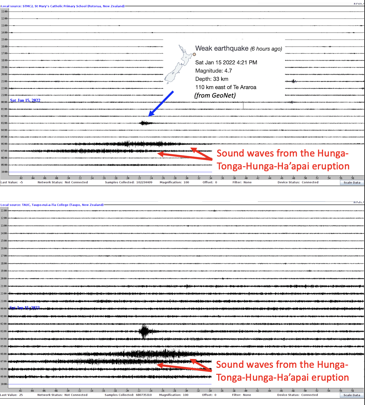
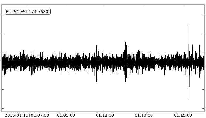
To give you an idea of the power of the eruption, please have a look at the attached image. Our school seismometers in Taupo Nui A Tia College and St Mary’s Catholic Primary In Rotorua recorded a cigar-like signal between 6 and 7.30 UTC. This equates to 7pm and 8.30pm local time, and is a recording of the the sound of the eruption, travelling through the air — not through the ground! — from Tonga to Taupo and Rotorua. At ~340 m/s, this sound took almost two hours to travel the ~2000 km from Tonga to Aotearoa.
By the way, you can also see the increase in noise on the station that started at 21.00UTC; this noise in Taupo (!) is caused by ocean waves from Cyclone Cody crashing on Aotearoa’s Eastern shores, and then shaking the ground all the way to Taupo…
Finally, as an exclamation point of the powers of Ranginui, Papatūānuku, and Rūaumoko, an Earthquake in Te Araroa (Magnitude 4.7) was also recorded at 3.22 UTC.
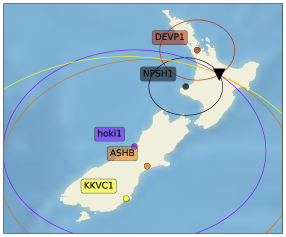
The “textbook” method to estimate the epicentre of an earthquake is based on the arrival time difference between the primary and secondary seismic wave. From this time difference, we can estimated the distance from the station to the earthquake; in other words, from a single station, we know the earthquake happened anywhere on a circle centered on the station, where the radius is the estimated epicentral distance. The intersection of at least three station’s circles provides an estimate of the epicentre.
circles centered on each seismic station represent the epicentral distance to an earthquake. The intersection of all circles is at the epicentre.
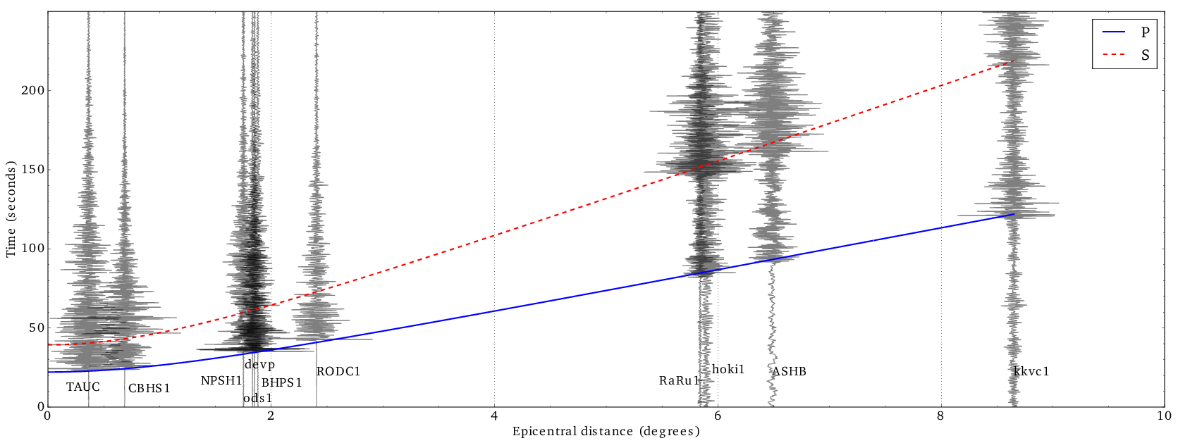
But how do we get the radius for each circle? In the figure below, you can see the seismograms from several of the Ru seismic stations for an earthquake near Rotorua, plotted as a function of their distance to Rotorua. The red and blue curves are predicted arrival times for the primary and secondary wave, based on a spherically symmetric earth. We made this figure for a publication in the European Journal of Physics, but the jupyter notebook that generates these figures is available here.
The distinct arrivals of the primary and secondary wave are matched with the arrival time curves predicted for a spherically symmetric earth.
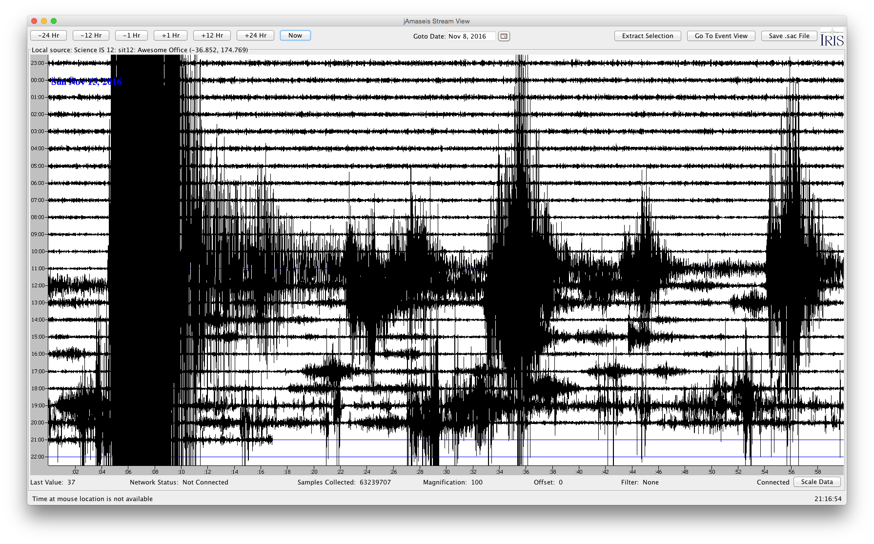
This is a screenshot of the seismic recordings at Birkenhead Primary School, on November 13th, 2016.
Shortly after midnight, last night, a severe earthquake struck the South Island. The full extent of the damage is not clear yet, and of course the members of the Ru network think about those affected by this event.
The seismic networks computed the thrust motion on the fault in a matter of minutes, and in this case the motion on the fault warranted a tsunami warning.
The New Zealand Herald features an article with the first reactions from geonet scientists. The mention of the Hope Fault is interesting. This fault is the southern-most fault of the Marlborough Faults (as far as we know!), which extend from the Alpine Fault. However, both Geonet and the USGS indicate a more southern placement of the epicentre. Besides, the Hope Fault is a strike-slip fault, whereas this event was a thrust fault! We at Ru wouldn’t be surprised if this event was slip (or slips, plural) on a combination of faults. In any case, there will much to learn from this event in the coming time. A discussion about the complexity of the tectonics in this area has already been posted on the USGS website.
Meanwhile, you can expect hundreds of aftershocks to fill your station helicorder screens in the coming days and weeks. If you get this message on Monday November 14th (local New Zealand time), you can see much of the action on our network page, similar to the image at the top of this post from Birkenhead Primary School.
Last week we welcomed James Hargest College, Invercargill and Koraunui School, Lower Hutt to the Ru Network. James visited the schools to help with set-up and run some Earthquake location demos with students. We were met in Invercargill by a reporter for an article in the Southland Times.
Some photos from the day at Koraunui.
Thanks to all the students and teachers at both schools. We hope you enjoy using the seismometer to explore the Earth!
Earthquakes occur on fault lines. Faults are fractures in the Earth’s crust formed by stress due to tectonic plates grinding together. When the stress builds high enough, the crust ruptures, causing an earthquake and a fault is formed. The Earth’s crust is displaced on either side of the fault.
Labelled Fault. (n.d.). Retrieved March 22, 20016, from http://earthquake.usgs.gov/learn/kids/eqscience.php
Faults are often only observed under the Earth. But we can sometimes see them on land too!
Go to google maps (or google Earth) and locate the following features:
Wallace Creek, California (USA). You can input the coordinates 35.27189, -119.82741 . Identify the rivers and look at their shape. Are the river shaped as you expect? Could a fault have changed the river shape/direction? Can you identify the fault?
Alpine Fault (New Zealand). Input the following coordinates: -42.6834, 171.5686 and zoom out.
Look at Earth features that stop abruptly. Can you identify the famous Alpine Fault? The Alpine Fault created the Southern Alps. How do you think the Earth moved along the fault to create the Alps?
Take a look at the East African Rift Valley (input coordinates 6.462, 37.908 and zoom out (really far). Can you see the rift stretching from Ethiopia to Mozambique? Here plate tectonics are acting to split one plate into two new ones. Can you think how faults might allow a valley like this to form? What might Africa look like in another 30 million years? Look at the shape of the Great Lakes along the rift valley (Lake Turkana, Lake Malawi). Can you think why they might be elongated?
The Ru workshop took place on the 27th-29th January 2016. It was great to bring a group of people together with such passion and enthusiasm for teaching, to share ideas and contribute towards the seismometers in schools program.
Day 1 took place at the University of Auckland’s City Campus. The morning revolved around the Auckland Lablet; Physics experimentation on an Android tablet. There were demonstrations to showcase Lablet being used record and analyse several physics experiments and some very useful ideas came out of the discussion.
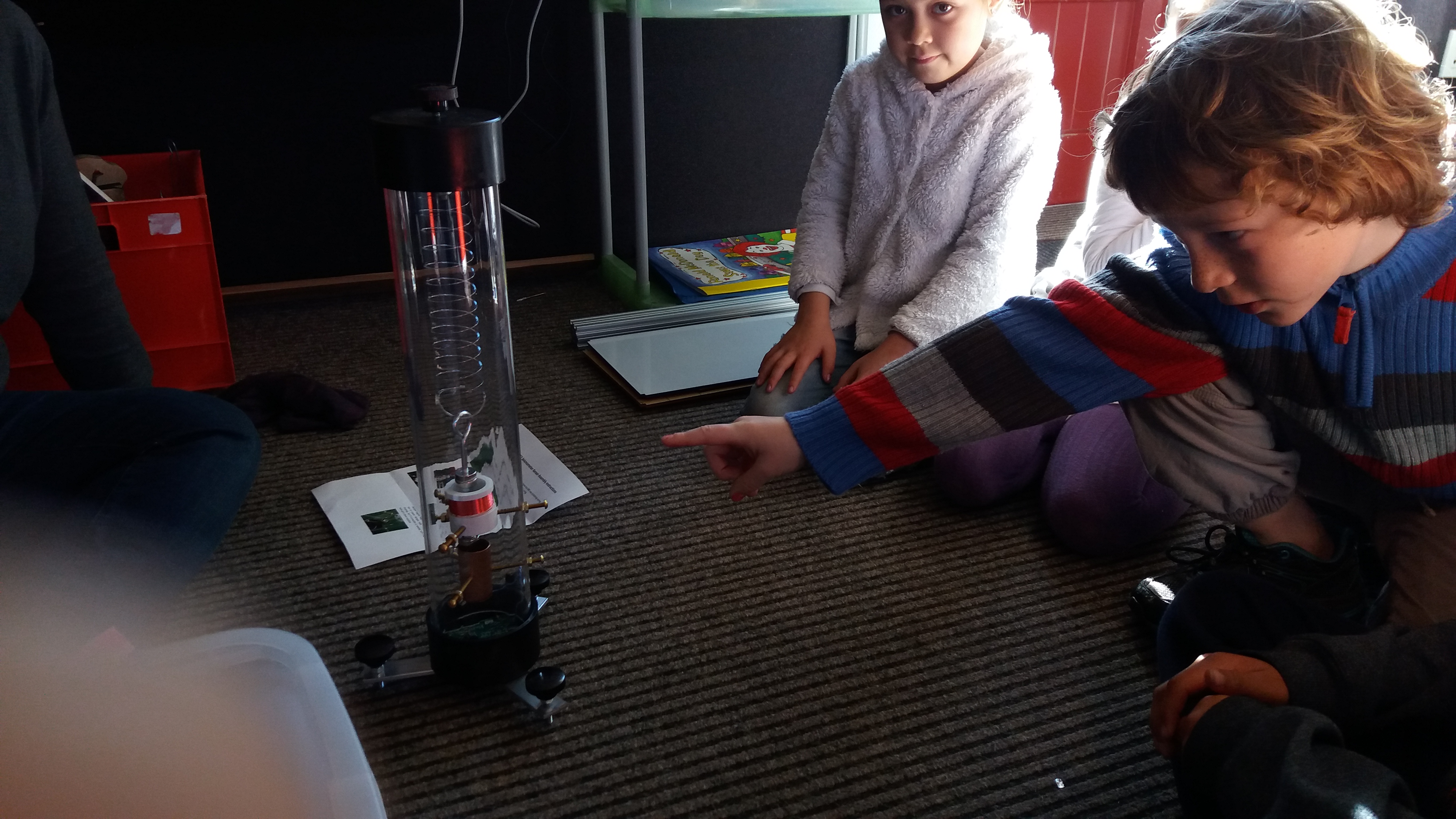
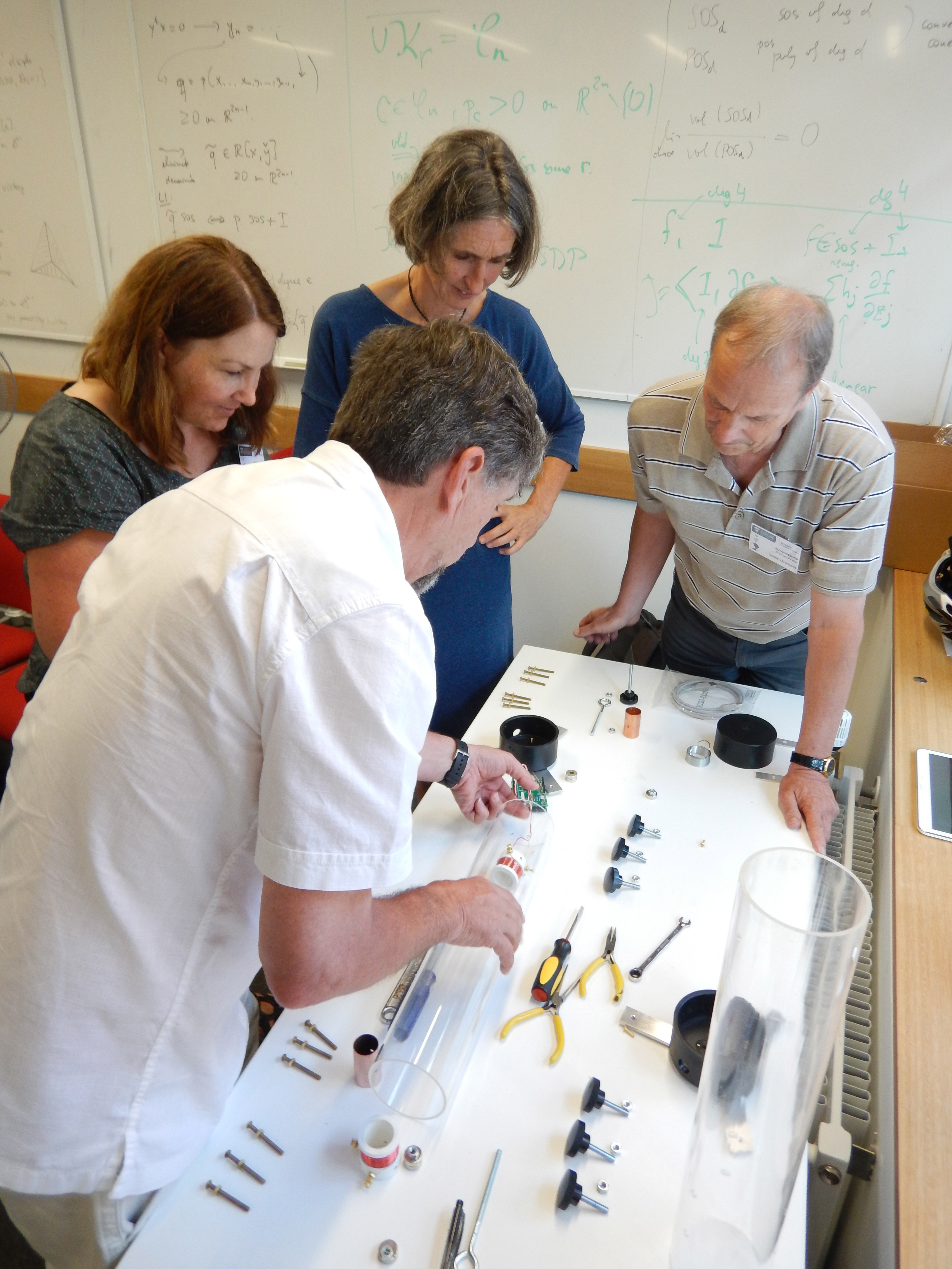
In the afternoon, the group were able to get their hands on the TC-1 Seismometer and built four from scratch. This showed just how simple it can be to construct the TC-1 and it was a great success when all four completed devices recorded data without a hitch.
Ted and team assembling a TC-1
There were several excellent talks over the rest of the afternoon. It was particularly interesting to hear (and see) how Jonathan had utilized an Arduino (a key component of the TC-1), to run a weather station.
Day 2 was spent on Waiheke Island. There were some great presentations by Dan Hikuroa, Caroline Little, Katrina Jacobs, Glenn Vallender, Michelle Salmon and Martin Smith. The day was nicely rounded off with some fantastic refreshments.
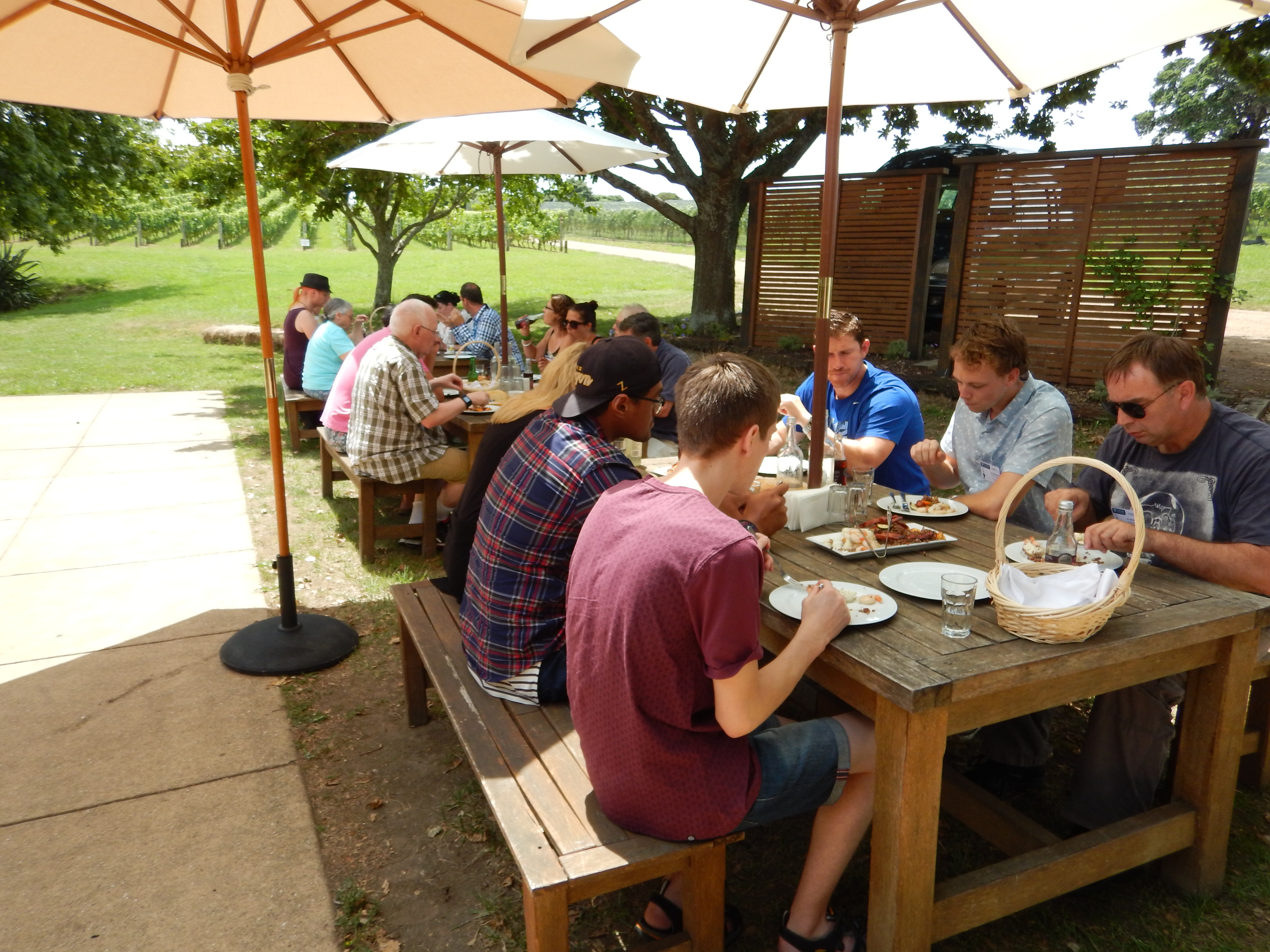
Great food on Waiheke
The highlight of Day 3 was undoubtedly the field trip to Rangitoto Island. The weather was excellent and although it was quite a hike up to the top, it was universally enjoyed. It was great to have Dan along as a guide to share his knowledge of the geology of the island and it was particularly interesting to explore the lava tubes.
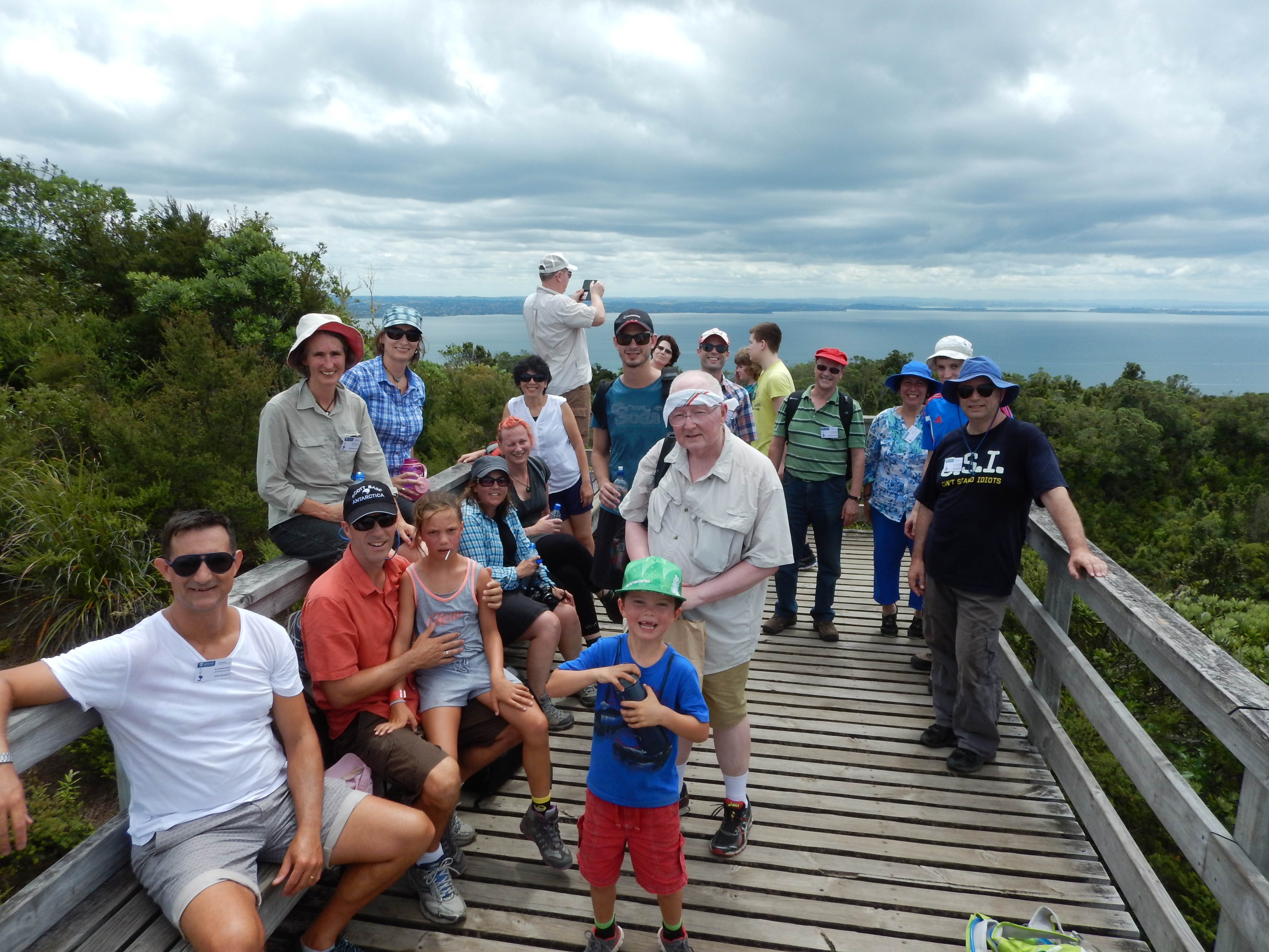
Ru on Rangitoto
Overall the workshop had a great turnout. We hope everyone enjoyed the three days and gained some ideas and insights that will be helpful in their schools.
The TC-1 seismometers in the Ru network are continuously recording small vibrations of the Earth. When these vibrations are seen on a seismogram they are called ‘noise’. Recently, we have been extracting useful information from the noise recorded by TC-1 seismometers in the Ru network using a technique called seismic interferometry.
Random vibrations of the Earth are seen as noise on a seismogram.
Noise can be thought of as a collection of seismic waves of different frequencies all stacked on top of each other to create a somewhat random signal–the same as sound noise, but with a much lower, inaudible average frequency. Because New Zealand is an island country surrounded by large oceans, a significant component of the low frequency noise comes from the interaction of the ocean with the seafloor and the land. Seismic interferometry analyses this noise and reveals evidence for surface waves generated by such a source which propagate through the Earth.
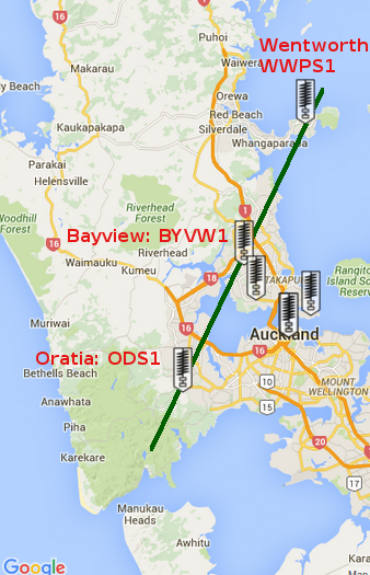
Ru stations in Auckland used for the seismic interferometry. Ocean noise from the west coast that is recorded at all three stations will travel along the green line.
The stations best suited for this analysis are those in coastal regions which form a near straight line between coasts when connected, such as those at Oratia District School (ODS), Bayview Primary School (BYVW), and Wentworth Private School (WWPS). The coastal environment of the Tasman Sea on the west of New Zealand is known to have higher energy than that on the east coast, so surface waves generated by the ocean-land interaction on the west coast which propagate east should be recorded in the seismic noise. And that’s exactly what the seismic interferometry with this data has revealed!
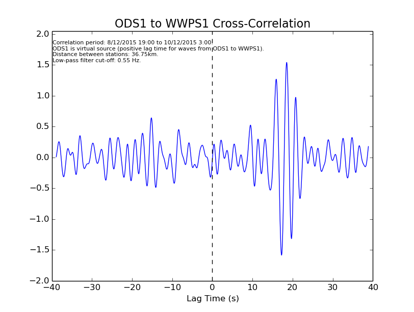
Oratia to Wentworth cross-correlation (33 hours). A low-pass digital filter with a cut-off frequency of 0.55 Hz was applied to the data in these analyses to remove significant influence from higher frequency noise, as the typical frequency of ocean noise is below 1 Hz.
The figure above shows the same as what you would see when looking at a normal seismogram, with time on the x-axis and amplitude of the signal on the y-axis. However, on the positive side of the x-axis, this plot shows Wentworth’s recording of an “earthquake” which occurred at 0 seconds at Oratia (and vice versa for a negative lag time). Of course, an earthquake never actually happened, but the cross-correlation uses the recorded noise over a long period to show what the signal might look like if an earthquake did occur (this is why ODS1 is the “virtual” source). The large peak at a time of about +15 to +25 s shows that a large component of the noise recorded at Wentworth takes 15-25 seconds to travel the distance from Oratia. The distance between the stations is 36.75 km, so waves which take 15-25 s to travel between Oratia and Wentworth propagate at about 1.5-2.5 km/s, a typical velocity for surface waves! A region of higher amplitude at -15 s to -25 s probably indicates surface waves travelling in the opposite direction, from the east coast to the west coast.
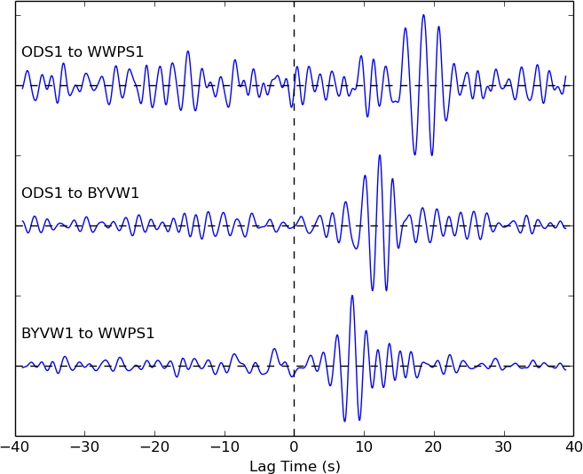
Similar results are obtained by cross-correlating the data between Oratia and Bayview, and Bayview and Wentworth. Since Bayview is at approximately the halfway point of the distance between Oratia and Wentworth, these two cross-correlations show the large peak at about half the lag time.
Cross-correlations of all three stations shown on the map above. The 2nd is over a period of 77 hours, and the third is over 79 hours.
While seismic interferometry can be used by seismologists to investigate properties of the subsurface (e.g. seismic wave velocities), our positive results demonstrate that data from the TC-1 seismometers in the Ru network is capable of being analysed in the same way as data from dedicated research-grade seismometers.
Thanks to all the station managers who have sent us their data, including those whose stations are not mentioned here (it’s a work in progress!).
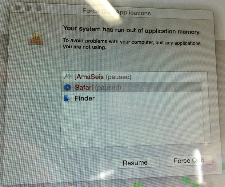
Unlike on Windows or Mac OS, jAmaSeis does not autodetect the serial port where a seismometer is connected on Linux. To run jAmaSeis on Linux, the jAmaseis.jar file must be started from the terminal with the correct serial port passed as a parameter. For the Arduino in the TC-1, this port will be /dev/ttyACM0 (or sometimes 1,2,3… instead of 0). The command to start jAmaSeis is:
It should also be noted that the Arduino drivers must be installed to read data sent by the TC-1. The easiest way to do this is by installing the Arduino IDE which will automatically install the appropriate drivers.
Since jAmaSeis is written in Java, a Java runtime environment must also be installed to run the .jar file. For example, OpenJDK.
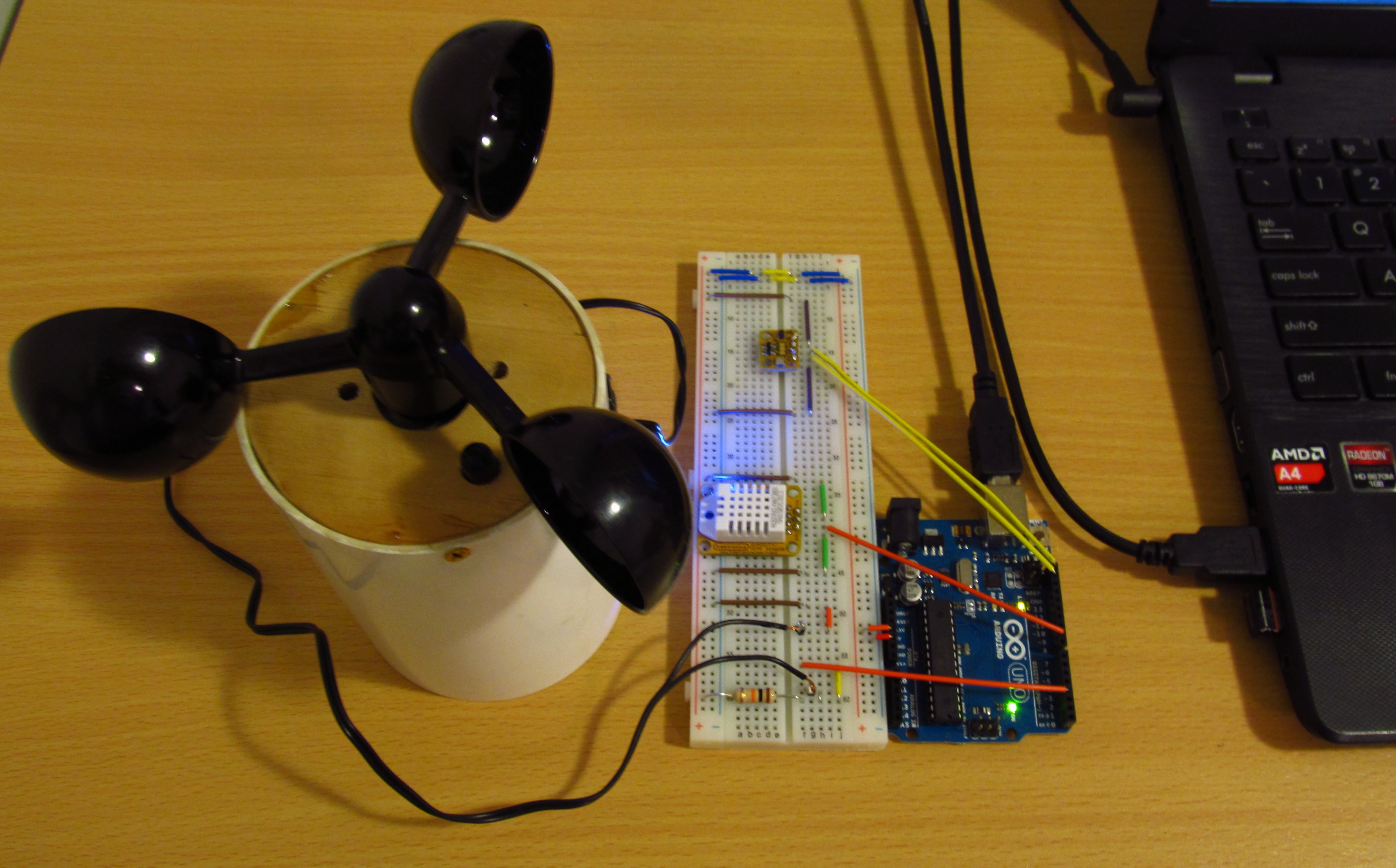
This Arduino ‘weather station’ acts as an example of the functionality of the Arduino microcontroller (which is used in the TC-1). It was presented at the recent Ru workshop as an “Arduemo” (!?) and is a nice little project for those with little or no experience in wiring or coding the Arduino. Here is a picture showing the layout of the circuit:
Arduino weather station with temperature, humidity, and pressure sensors as well as an anemometer to measure wind speed.
The temperature/humidity and pressure sensors are Arduino-compatible modules from freetronics, while the anemometer is ‘home-made’ from two ball bearings in a brass casing with a steel shaft and windcups (see specifications). The anemometer sensor is a magnetic reed switch from a bike computer, so the Arduino simply watches for when the switch is opened and closed. A closer look at the individual components and wiring of the circuit can be found here.