Category Archives: Uncategorized

The Ru Network on a pcDuino

A pcDuino is a ‘microcomputer’ which works the same as a normal desktop computer but is many times smaller. pcDuinos integrate well with the arduino board currently used in the TC-1 seismometer, so they make  a cost-effective alternative for computers in the Ru network.

The pcDuino microcomputer. The wires connected are power and HDMI output (right) as well as keyboard, mouse, and TC-1 (via USB hub). The length of the board is about 12cm.

The pcDuino runs the Linux-based operating system Lubuntu, which supports both the jAmaSeis and PyjAmaSeis software. Work is currently being done on the pcDuino and the software it runs so that we can use them in the Ru network sometime in the future.

A pcDuino running the PyjAmaSeis software.

PyjAmaseis

PyjAmaSeis is free software to record, display and process seismic data from your seismometer attached to a computer. The first version was developed by Saketh Vishnubhotla as part of his 4th year BTech (Hons) project at the University of Auckland.

PyjAmaSeis was inspired by jAmaseis (which was developed based on the succesful AmaSeis software), and is written in Python, a versatile programming language with interpreters available across operating systems.

Screenshot of PyjAmaSeis version 1.0 running on a pcDuino (see pcDuino and Linux category).

PyjAmaSeis uses a lot of the features developed as part of obspy, and we hope to develop a graphical user interface for teachers and students in the near future.

Workshop in Auckland, January 27th-29th, 2016

John Milne's Lamp post seismometer

January 27th:

Registration starts at 8.30am, outside room 412, located on the 4th floor of the Science Centre, building 303, 38 Princes St.,  Auckland. Easiest car parking is under the Owen Glenn building.

Room 412, building 303:

  • 9-9.30: Welcome and introductions
  • 9.30-10.30: Intro to Lablet, plus Lablet demo circuit: Doppler, Lift, big G, Aliasing. How to get Lablet at the google play store.
  • 10.30-11.00: Morning tea (basement foyer, 303)
  • 11.00-12.00: Stage 1 lab activity on the trajectory of a thrown ball
  • 12.00-12.30: Lablet discussion
  • 12.30-13.30: Lunch  served in the basement foyer of the Science Centre
  • 13:30-14.30: The anatomy of the TC1 seismometer with Ted Channel, Kasper van Wijk and James Clarke
  • 14.30:15.00: TC1 discussion about all the previous
  • 15.00-15.30: Afternoon tea  (basement foyer, 303)
  • 15.30-16.15: The arduino environment (as part of the TC1 and beyond) with live demos (“arduemos?”) by Martin Smith and Jonathan Simpson
  • 16.15-16.45: An introduction of Jamaseis by John Taber, IRIS
  • 16.45- 17.15: Wrap-up discussion

January 28th (to be held on Waiheke):

Meet at 8.30am at the Auckland Ferry terminal.
9.00 am Auckland – Waiheke
9.45 am Matiatia – The Goldie Room
10.00 am Arrive The Goldie Room

  • 10.00-10.30: Welcome, and discussion on indigenous knowledge in seismology, geosciences, and science in general, led by Dan Hikuroa
  • 10.30-11.00: Geonet: New Zealand’s seismic network by the professionals in seismology, Caroline Little
  • 11.00-11.15: Morning tea
  • 11.15-11.30: Katrina Jacobs on SARndbox
  • 11.30-12.00: An example of earthquake location by Kasper van Wijk and James Clarke; from primary school to secondary school level
  • 12.00-12.45: Discussion on the current use of Ru in the classroom, the links to plate tectonics, NZ geosciences and NCEA, led by Glenn Vallender
  • 12.45-14.00: Lunch provided
  • 14.00-14.30: School seismology lessons learned from overseas, led by Michelle Salmon, Australian National University
  • 14.30-15.00: Break out session to discuss in small groups all that was presented up to this point.
  • 15.00-15.30:  Everything looks good on a log scale, by Martin Smith on the Gutenberg-Richter and Omori’s Law for primary and secondary students
  • 15.30-17.00: Closing discussion with typical Goldie’s refreshments

5.20 pm The Goldie Room – Matiatia
5.50 pm Waiheke – Auckland
6.25 pm Arrive back in Auckland

January 29th (on Campus)

Room B05, Science Centre:

  • 9.00-9.45: IT challenges, led by Yvette Wharton and Mat Carr
  • 9.45-10.15: Pyjamaseis and pcduinos by Jonathan Simpson (powerpoint presentation)
  • 10.15- 10.30: Morning tea in the foyer of the basement in the Science Centre
  • 10.30-11.30: Breakout sessions by level about the road ahead. Primary schools with Ludmila Adam, Secondary schools with Kasper van Wijk, and Tertiary institutions with Dan Hikuroa
  • noon-5.15pm:  Field trip to Rangitoto, leave on the 12.15 ferry, lunch provided on the island, leaving Rangitoto at 4.30pm. Field guide

M5.8, 30 km north-west of Wanaka

On May 4, 2015, at 2:29:10 UTC, an earthquake with magnitude 5.8 occured 30 km north-west of Wanaka.  Most of the TC1 seismometers of the Ru network recorded the resulting seismic waves.  Check out the map below, where the epicentre of the quake is shown as a red dot, and the stations in the Ru network are shown as black triangles.

RUstationmap

The records of the earthquake motion are called seismograms.  Each “seismogram” is a record of the velocity of the earth at a particular time.  In the figure below, the seismograms are offset horizontally from the left of the graph.  This offset is the epicentral distance (distance from the epicentre) to each station.  The vertical time scale starts at the origin time of the earthquake.


section

There are two important things to notice about this figure.  First of all, Hokitika, Rangi-Ruru, and Ashburton museum stations are the closest to the earthquake and have very similar epicentral distances.   Therefore the the earthquake reaches them at close to the same time, and the stations are spaced close together on the horizontal axis.  Also, notice that these seismograms have large amplitudes and overlap each other.  By contrast, the two stations further away, in Auckland, record the earthquake at later times.  The amplitude recorded on these stations is also smaller, which makes sense because seismic waves spread out as they travel greater distances.

To see the waveforms more clearly, here is a simple plot of what all stations recorded.  Note that the vertical scale of the different plots is not consistent from plot to plot:

stream


Also note that these plots do not look the same.  This is the result of path effects.  To begin with, as seismic waves travel through the earth, the earth attenuates (makes smaller) certain frequencies more than others, and which frequencies it attenuates depends upon which path the quake travels.  Since the waves took different paths to make it to our different stations, the recorded earthquakes look different.  But this is only part of the picture.  Notice that at the two stations which are further away, the seismograms are longer.  In addition to the primary wave (the fastest, which arrives first), there are other, slower waves that arrive later.  The further a station is from the epicentre, the longer it takes for all the waves to arrive, and therefore the recorded quake is longer.

And lastly, here’s a seismic section with data from our Taupo station included.  As you can see, it looks like the earthquake arrives a bit before it should.  The computer clock for this station was not accurate, which shows how important it is for professional seismologists to make sure their clocks are set right! (of course we at Ru understand that’s not always possible with the equipment we provide you).

taupo

Thank you to all the station managers who sent me data!  If you haven’t yet sent me your data, please do, and I can update the figures!

Embedding the Rū map in a web page

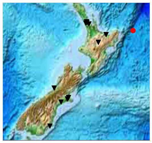
See this map at http://ru.auckland.ac.nz/the-network/.

The code

Insert the following “inline” where you want the map to appear. At the time of writing, the code was still in flux, but what you see here will be a functional subset of what may be available later.

<!-- rū map -->
<div id="ru_canvas"></div>
<style type="text/css">
@import url("https://nzseis.phy.auckland.ac.nz/map/css/ru_mapem.css");
</style>
<script src="https://maps.googleapis.com/maps/api/js"></script><script src="https://nzseis.phy.auckland.ac.nz/last50/js/ru_stations.js"></script><script src="https://nzseis.phy.auckland.ac.nz/map/geonet.php?mode=js"></script><script src="https://nzseis.phy.auckland.ac.nz/map/usgs.php?mode=js"></script><script src="https://nzseis.phy.auckland.ac.nz/map/js/ru_mapfunctions.js"></script><script src="https://nzseis.phy.auckland.ac.nz/map/js/ru_legend.js"></script><script src="https://nzseis.phy.auckland.ac.nz/map/js/ru_mapinitem.js"></script><script type="text/javascript">
// <![CDATA[
var ru_options = {
"centreonstation": false,
"width": "640px",
"height": "640px",
"zoom": 5,
"iconscale": 1,
"fontscale": "100%",
"showusgs": true,
"showgeonet": true,
"showlegend": true,
"lat": -41.0,
"lon": 174.0,
"canvas": document.getElementById('ru_canvas'),
};
RU_ICON_SCALE = ru_options.iconscale;
RU_FONT_SCALE = ru_options.fontscale;
google.maps.event.addDomListener(window, 'load', ru_initialize());
// ]]>
</script>
<!-- /rū map -->

A number of parameters can be configured to change the way the map is displayed -these are wrapped up in a javascript object (ru_options).

The paramaters

centreonstation
false or the short name of a station in the Rū family. If false, then the map will centre on the latitude and longitude specified using “lat” and “lon”. If a station is specified, then the map will centre on the latitude and longitude recorded for that station.

width and height
String literals that are assigned to the respective style properties of the map canvas. You could specify a dimension in pixels, a percentage, or whatever units CSS allows. The posts associated with stations in this web site, use “474px” for height and width.
“100%” (with appropriate styling of the canvas element) could be used to fill a viewport.

zoom
An integer between 1 and 20, representing the zoom steps the Google Maps API allows. 5 or 6 is good for a view of the whole of New Zealand, 17 is good for a view of a building in its context.

iconscale
A positive and non-zero decimal value used to vary the scale of the icons used as map markers. All markers are scaled by this value which can be used to make the map more legible at different sizes.

fontscale
A string literal added as a font-size style property to the legend (if it is visible). This can be used to adjust how the legend looks at different sizes.

showusgs, showgeonet and showlegend
True or false. These give you control of the visibility of the various information layers available.

lat and lon
A Latitude and longitude that will be used to centre the map if centreonstation is false. The default provided is near the centre of New Zealand (-41.0, 174.0).

canvas
Used to pass the element used as the map canvas to the initialisation function -if you name the container differently (ie. not ru_canvas), then change the id inside the getElementById expression.


M6.5, 155 km east of Te Araroa

On November 16 2014, at 22:33:17 (UTC), an earthquake with magnitude 6.5 occurred some  155 km east of Te Araroa:
The stations of the Ru network recorded the resulting seismic waves, displayed  in the figure below. The so-called “seismogram” for each station shows the propagation of the vibrations caused by the quake:
The horizontal position of each seismogram represents the distance from the epicentre to each station. The vertical time scale starts at the origin time of the earthquake.

RUstationmap
Black triangles indicate the location of the Ru stations. The red circle is the epicentre of the M6.5 earthquake. Click on the figure to see a larger version.

For example, it takes roughly 180 seconds for the first seismic wave to get to station kkvc1 in Kaikoria Valley, some 1200 km from the epicentre. This means the average speed of this primary (or P-)wave is 6.7 km/s! Over this relatively short distances,  you can almost draw a straight line through the onsets of energy on each seismogram, showing that the wave speed varies only by per cents  in the subsurface under our network.

gisborne2014
Seismograms of each Ru station, organised by distance from the Earthquake. Click on the image to enlarge.

Also, notice how the seismograms change from station to station. For the close ones, the waves are bunched up in a relatively short time span, whereas for those stations with a greater epicentral distance, the “wave train” is longer.  It turns out that in addition to the primary wave, there are other, slower, waves in this wave train. These include secondary (or S-)waves, and surface waves.

Finally, we should mention that the amplitudes of each seismogram are equalised to show the arrival times the clearest.  In reality, the vibrations recorded closer the epicentre are much larger than those farther away.


Assembling the case for your TC1

Below you find detailed instructions on the assembly of an aluminium and plexi-glass case for the TC1 seismometer. It was successfully tested by an 11-year old volunteer from Oratia District School (thank you, Hayden!)

Click on the images for more detail and a short description.Once assembled, it is recommended to fasten the completed case to a wall.


Thank you Mark,  Trevor, Steve and all others from the Science and Engineering Workshop!