With great pleasure we welcome Woodford House to the Ru network. James Clarke visited the school, and we are very pleased to hear all the positive feedback coming from there! As an aside, the network of schools has grown to over 30 stations. To see the recordings from these schools, you can visit the live rumblings page.
All posts by kvan637
A jupyter notebook to illustrate earthquake location
The “textbook” method to estimate the epicentre of an earthquake is based on the arrival time difference between the primary and secondary seismic wave. From this time difference, we can estimated the distance from the station to the earthquake; in other words, from a single station, we know the earthquake happened anywhere on a circle centered on the station, where the radius is the estimated epicentral distance. The intersection of at least three station’s circles provides an estimate of the epicentre.
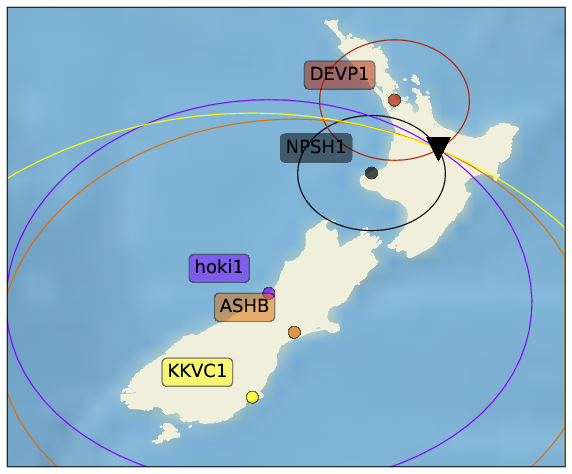
But how do we get the radius for each circle? In the figure below, you can see the seismograms from several of the Ru seismic stations for an earthquake near Rotorua, plotted as a function of their distance to Rotorua. The red and blue curves are predicted arrival times for the primary and secondary wave, based on a spherically symmetric earth. We made this figure for a publication in the European Journal of Physics, but the jupyter notebook that generates these figures is available here.
Severe earthquake NNE of Amberley, NZ
Shortly after midnight, last night, a severe earthquake struck the South Island. The full extent of the damage is not clear yet, and of course the members of the Ru network think about those affected by this event.
The seismic networks computed the thrust motion on the fault in a matter of minutes, and in this case the motion on the fault warranted a tsunami warning.
The New Zealand Herald features an article with the first reactions from geonet scientists. The mention of the Hope Fault is interesting. This fault is the southern-most fault of the Marlborough Faults (as far as we know!), which extend from the Alpine Fault. However, both Geonet and the USGS indicate a more southern placement of the epicentre. Besides, the Hope Fault is a strike-slip fault, whereas this event was a thrust fault! We at Ru wouldn’t be surprised if this event was slip (or slips, plural) on a combination of faults. In any case, there will much to learn from this event in the coming time. A discussion about the complexity of the tectonics in this area has already been posted on the USGS website.
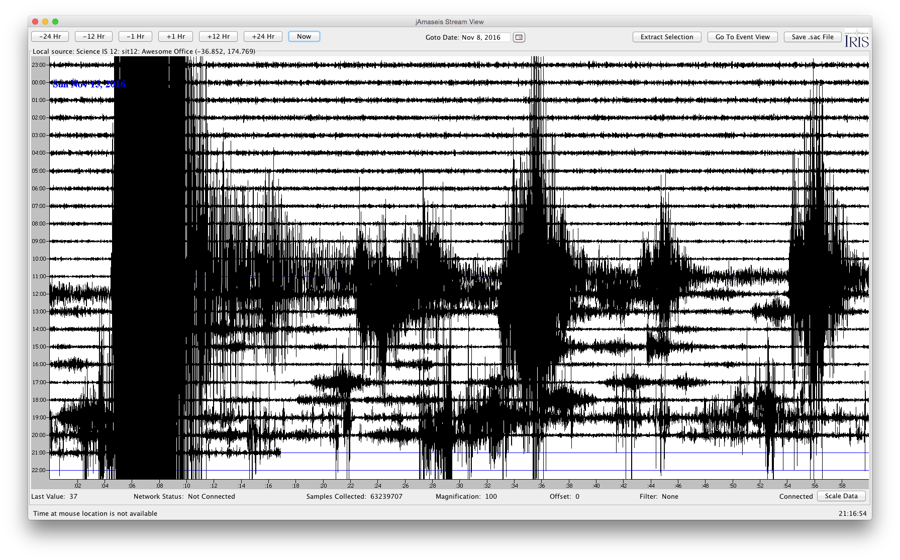
Meanwhile, you can expect hundreds of aftershocks to fill your station helicorder screens in the coming days and weeks. If you get this message on Monday November 14th (local New Zealand time), you can see much of the action on our network page, similar to the image at the top of this post from Birkenhead Primary School.
.
A report from our Workshop
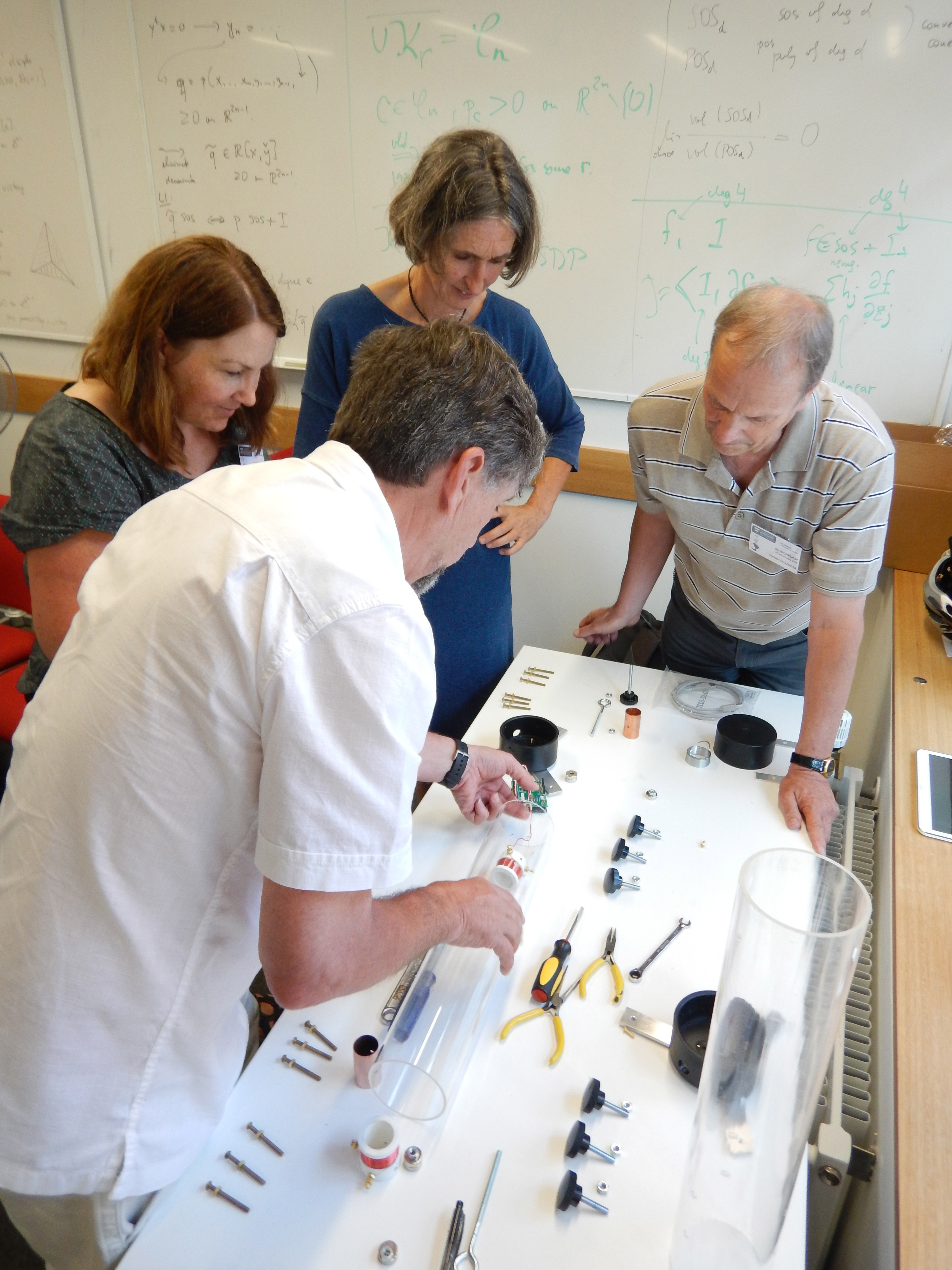
The Ru workshop took place on the 27th-29th January 2016. It was great to bring a group of people together with such passion and enthusiasm for teaching, to share ideas and contribute towards the seismometers in schools program.
Day 1 took place at the University of Auckland’s City Campus. The morning revolved around the Auckland Lablet; Physics experimentation on an Android tablet. There were demonstrations to showcase Lablet being used record and analyse several physics experiments and some very useful ideas came out of the discussion.
In the afternoon, the group were able to get their hands on the TC-1 Seismometer and built four from scratch. This showed just how simple it can be to construct the TC-1 and it was a great success when all four completed devices recorded data without a hitch.
There were several excellent talks over the rest of the afternoon. It was particularly interesting to hear (and see) how Jonathan had utilized an Arduino (a key component of the TC-1), to run a weather station.
Day 2 was spent on Waiheke Island. There were some great presentations by Dan Hikuroa, Caroline Little, Katrina Jacobs, Glenn Vallender, Michelle Salmon and Martin Smith. The day was nicely rounded off with some fantastic refreshments.
The highlight of Day 3 was undoubtedly the field trip to Rangitoto Island. The weather was excellent and although it was quite a hike up to the top, it was universally enjoyed. It was great to have Dan along as a guide to share his knowledge of the geology of the island and it was particularly interesting to explore the lava tubes.
Overall the workshop had a great turnout. We hope everyone enjoyed the three days and gained some ideas and insights that will be helpful in their schools.

Workshop in Auckland, January 27th-29th, 2016
January 27th:
Registration starts at 8.30am, outside room 412, located on the 4th floor of the Science Centre, building 303, 38 Princes St., Auckland. Easiest car parking is under the Owen Glenn building.
Room 412, building 303:
- 9-9.30: Welcome and introductions
- 9.30-10.30: Intro to Lablet, plus Lablet demo circuit: Doppler, Lift, big G, Aliasing. How to get Lablet at the google play store.
- 10.30-11.00: Morning tea (basement foyer, 303)
- 11.00-12.00: Stage 1 lab activity on the trajectory of a thrown ball
- 12.00-12.30: Lablet discussion
- 12.30-13.30: Lunch served in the basement foyer of the Science Centre
- 13:30-14.30: The anatomy of the TC1 seismometer with Ted Channel, Kasper van Wijk and James Clarke
- 14.30:15.00: TC1 discussion about all the previous
- 15.00-15.30: Afternoon tea (basement foyer, 303)
- 15.30-16.15: The arduino environment (as part of the TC1 and beyond) with live demos (“arduemos?”) by Martin Smith and Jonathan Simpson
- 16.15-16.45: An introduction of Jamaseis by John Taber, IRIS
- 16.45- 17.15: Wrap-up discussion
January 28th (to be held on Waiheke):
Meet at 8.30am at the Auckland Ferry terminal.
9.00 am Auckland – Waiheke
9.45 am Matiatia – The Goldie Room
10.00 am Arrive The Goldie Room
- 10.00-10.30: Welcome, and discussion on indigenous knowledge in seismology, geosciences, and science in general, led by Dan Hikuroa
- 10.30-11.00: Geonet: New Zealand’s seismic network by the professionals in seismology, Caroline Little
- 11.00-11.15: Morning tea
- 11.15-11.30: Katrina Jacobs on SARndbox
- 11.30-12.00: An example of earthquake location by Kasper van Wijk and James Clarke; from primary school to secondary school level
- 12.00-12.45: Discussion on the current use of Ru in the classroom, the links to plate tectonics, NZ geosciences and NCEA, led by Glenn Vallender
- 12.45-14.00: Lunch provided
- 14.00-14.30: School seismology lessons learned from overseas, led by Michelle Salmon, Australian National University
- 14.30-15.00: Break out session to discuss in small groups all that was presented up to this point.
- 15.00-15.30: Everything looks good on a log scale, by Martin Smith on the Gutenberg-Richter and Omori’s Law for primary and secondary students
- 15.30-17.00: Closing discussion with typical Goldie’s refreshments
5.20 pm The Goldie Room – Matiatia
5.50 pm Waiheke – Auckland
6.25 pm Arrive back in Auckland
January 29th (on Campus)
Room B05, Science Centre:
- 9.00-9.45: IT challenges, led by Yvette Wharton and Mat Carr
- 9.45-10.15: Pyjamaseis and pcduinos by Jonathan Simpson (powerpoint presentation)
- 10.15- 10.30: Morning tea in the foyer of the basement in the Science Centre
- 10.30-11.30: Breakout sessions by level about the road ahead. Primary schools with Ludmila Adam, Secondary schools with Kasper van Wijk, and Tertiary institutions with Dan Hikuroa
- noon-5.15pm: Field trip to Rangitoto, leave on the 12.15 ferry, lunch provided on the island, leaving Rangitoto at 4.30pm. Field guide
Slinky Seismometer in Estes Park, Colorado (USA)
Below you can see a video of students from Estes Park, Colorado, who worked with Ted Channel and Vera Schulte Pelkum on building, installing, recording and analysing earthquakes. Well done!
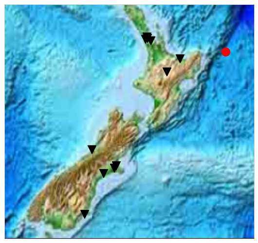
M6.5, 155 km east of Te Araroa
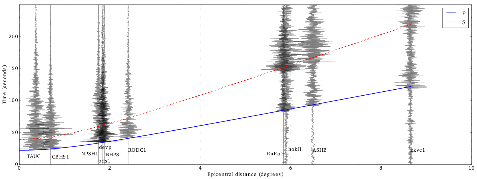
On November 16 2014, at 22:33:17 (UTC), an earthquake with magnitude 6.5 occurred some 155 km east of Te Araroa:
The stations of the Ru network recorded the resulting seismic waves, displayed in the figure below. The so-called “seismogram” for each station shows the propagation of the vibrations caused by the quake:
The horizontal position of each seismogram represents the distance from the epicentre to each station. The vertical time scale starts at the origin time of the earthquake.
For example, it takes roughly 180 seconds for the first seismic wave to get to station kkvc1 in Kaikoria Valley, some 1200 km from the epicentre. This means the average speed of this primary (or P-)wave is 6.7 km/s! Over this relatively short distances, you can almost draw a straight line through the onsets of energy on each seismogram, showing that the wave speed varies only by per cents in the subsurface under our network.
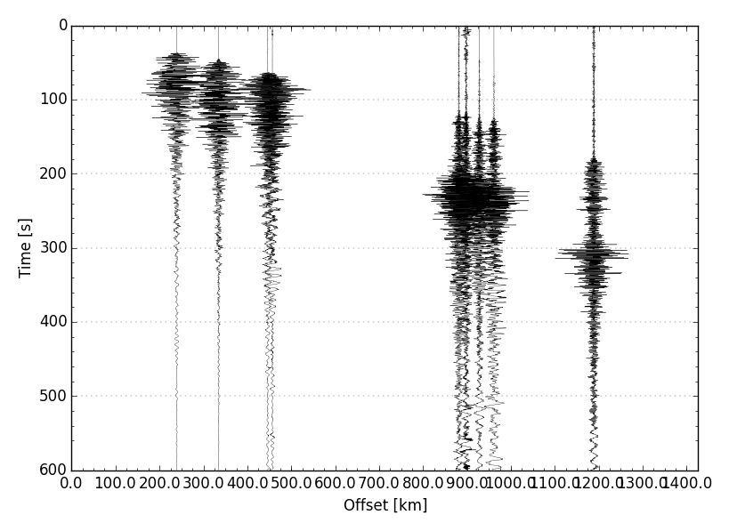
Also, notice how the seismograms change from station to station. For the close ones, the waves are bunched up in a relatively short time span, whereas for those stations with a greater epicentral distance, the “wave train” is longer. It turns out that in addition to the primary wave, there are other, slower, waves in this wave train. These include secondary (or S-)waves, and surface waves.
Finally, we should mention that the amplitudes of each seismogram are equalised to show the arrival times the clearest. In reality, the vibrations recorded closer the epicentre are much larger than those farther away.
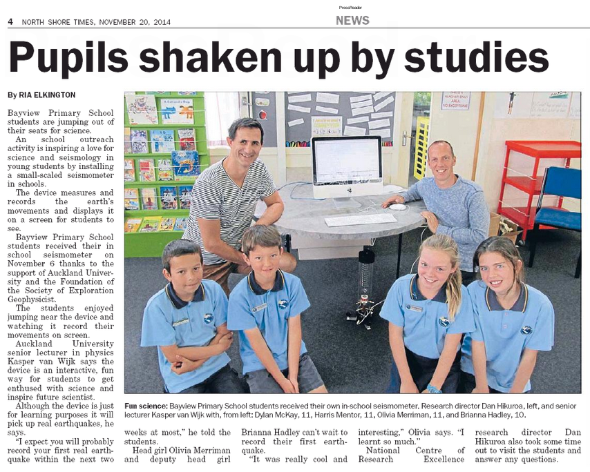
Ru in the North Shore Times
How to extract data from jamaseis
Assembling the case for your TC1
Below you find detailed instructions on the assembly of an aluminium and plexi-glass case for the TC1 seismometer. It was successfully tested by an 11-year old volunteer from Oratia District School (thank you, Hayden!)
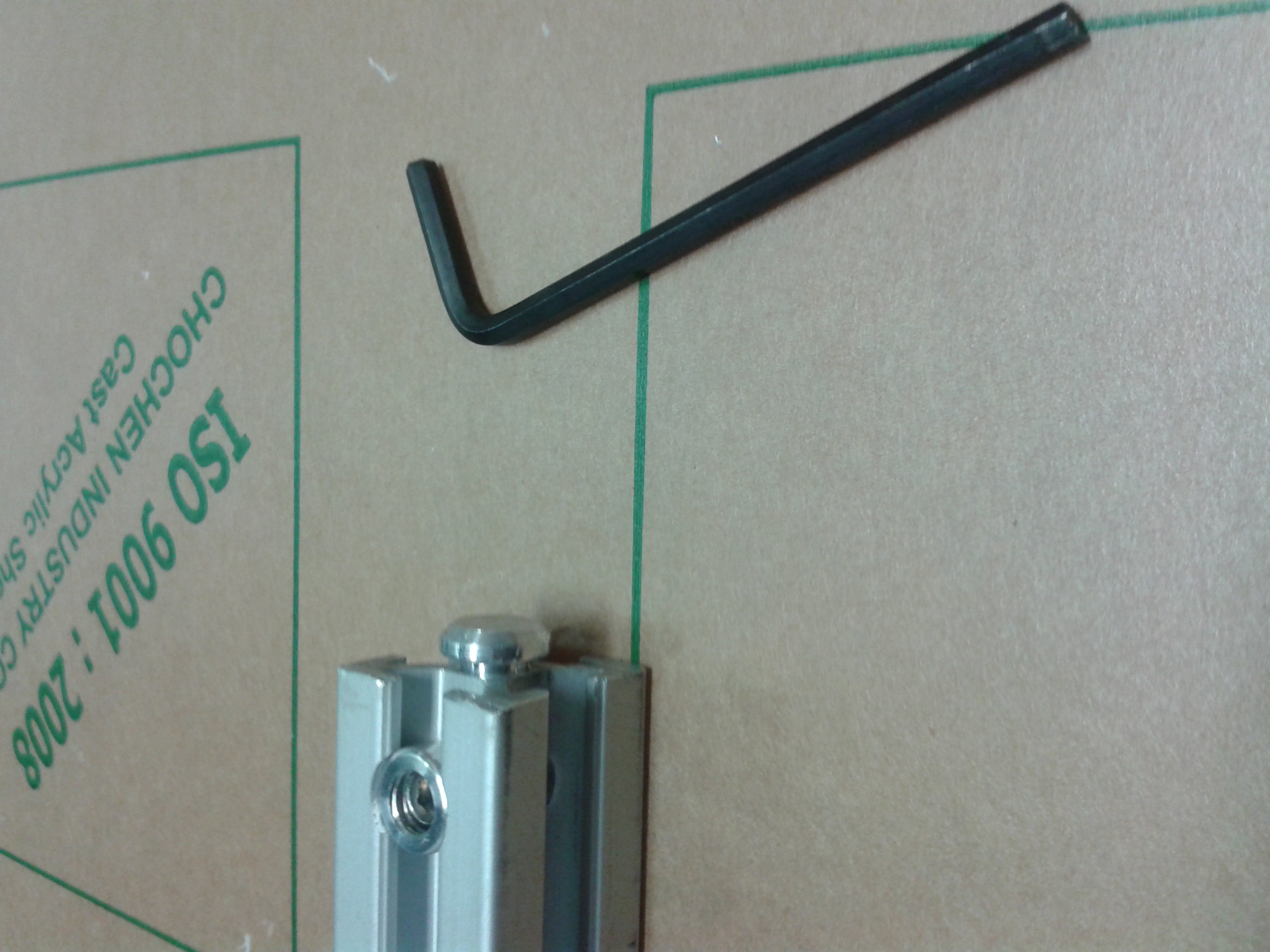
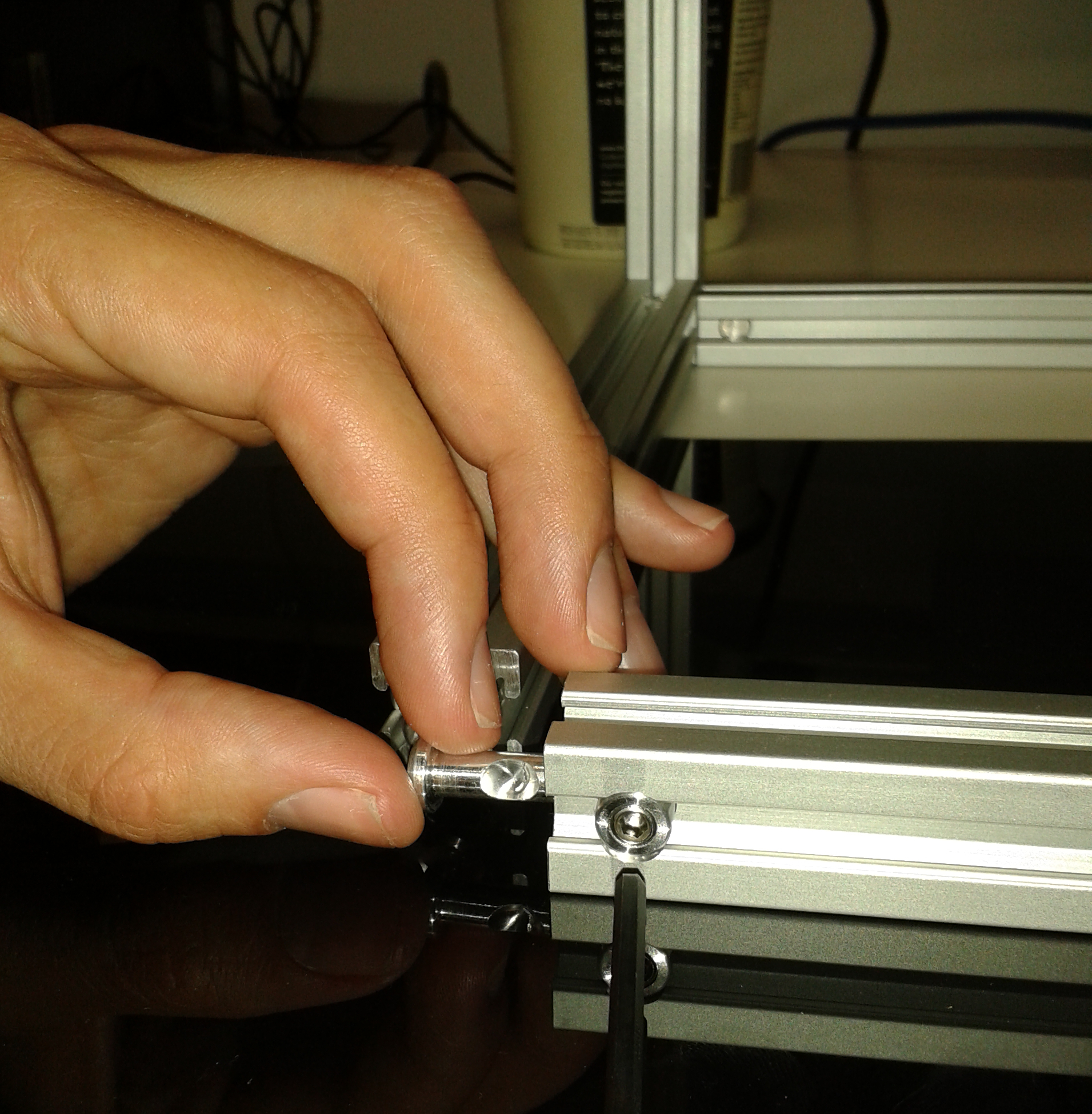
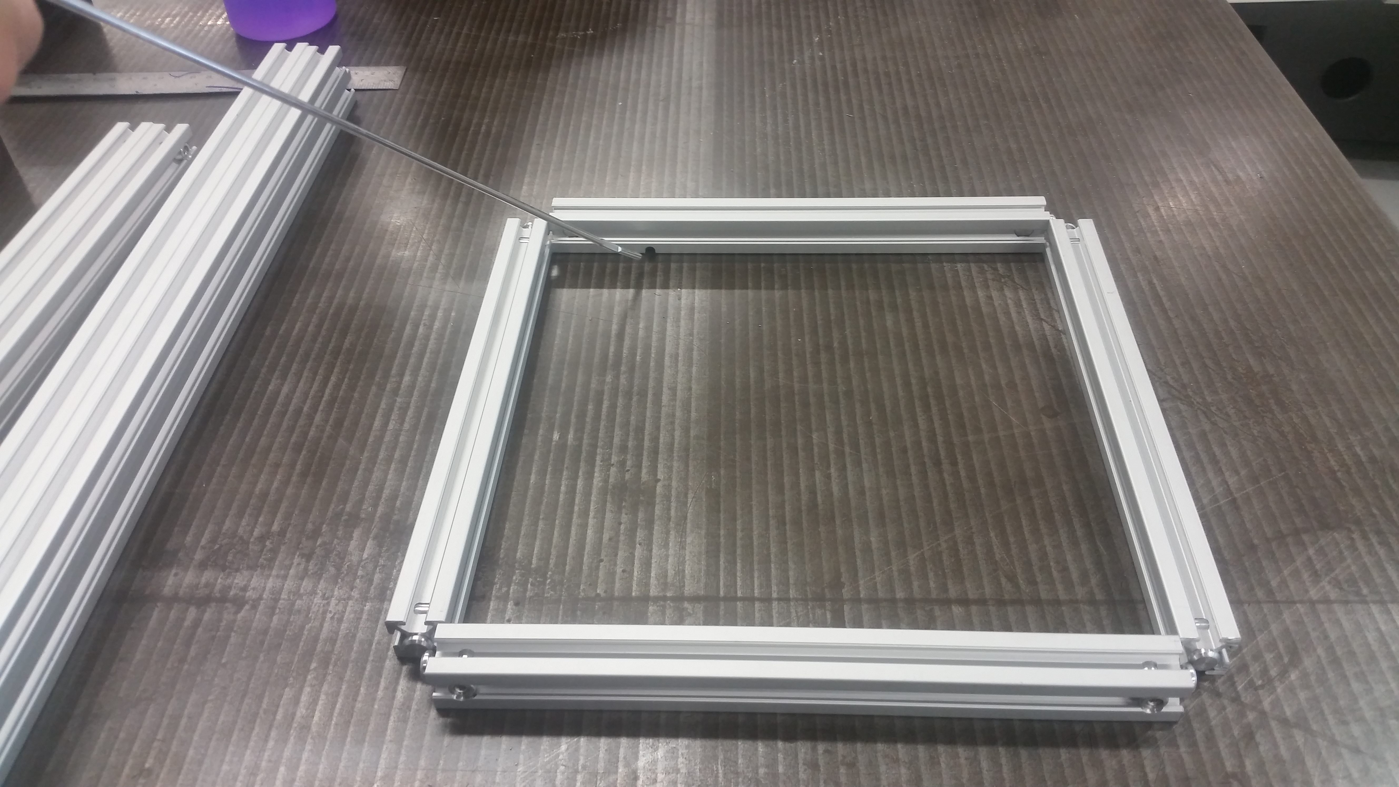
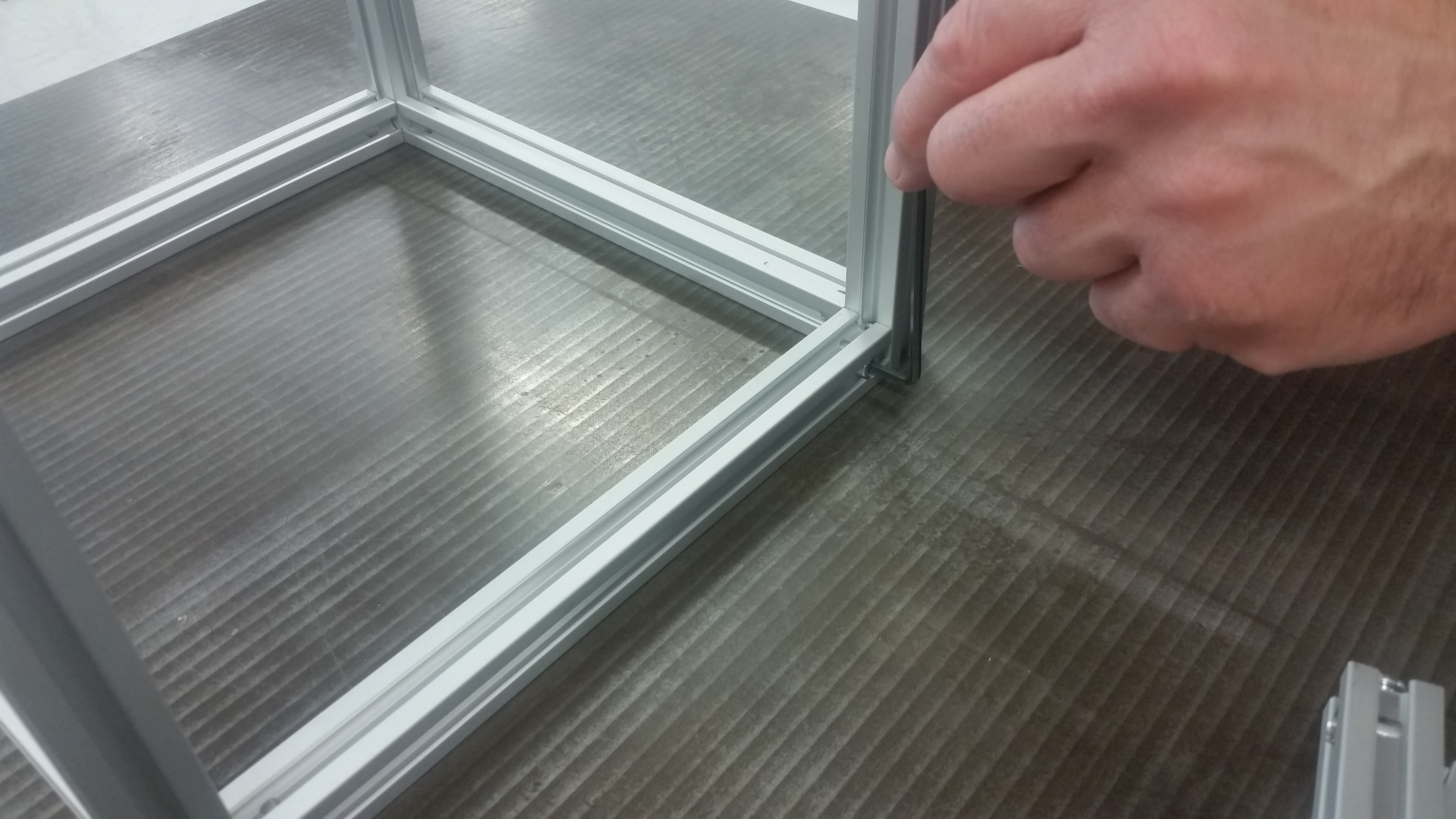
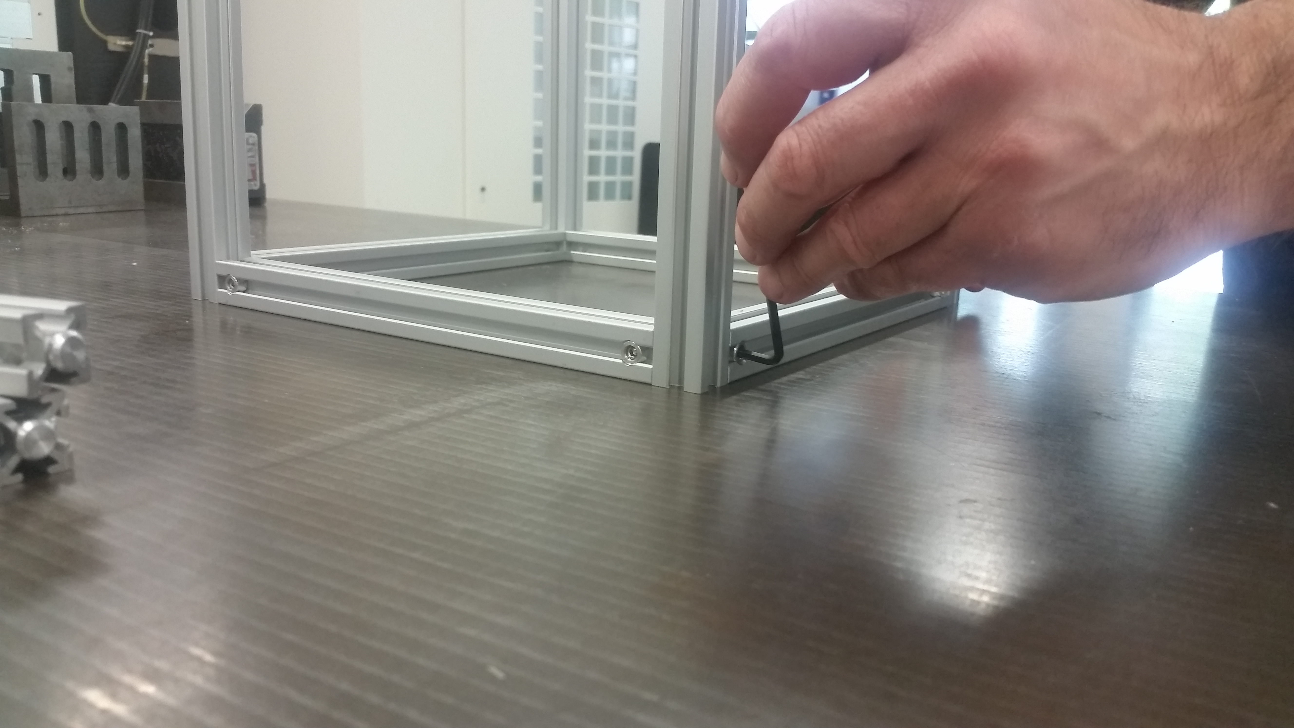
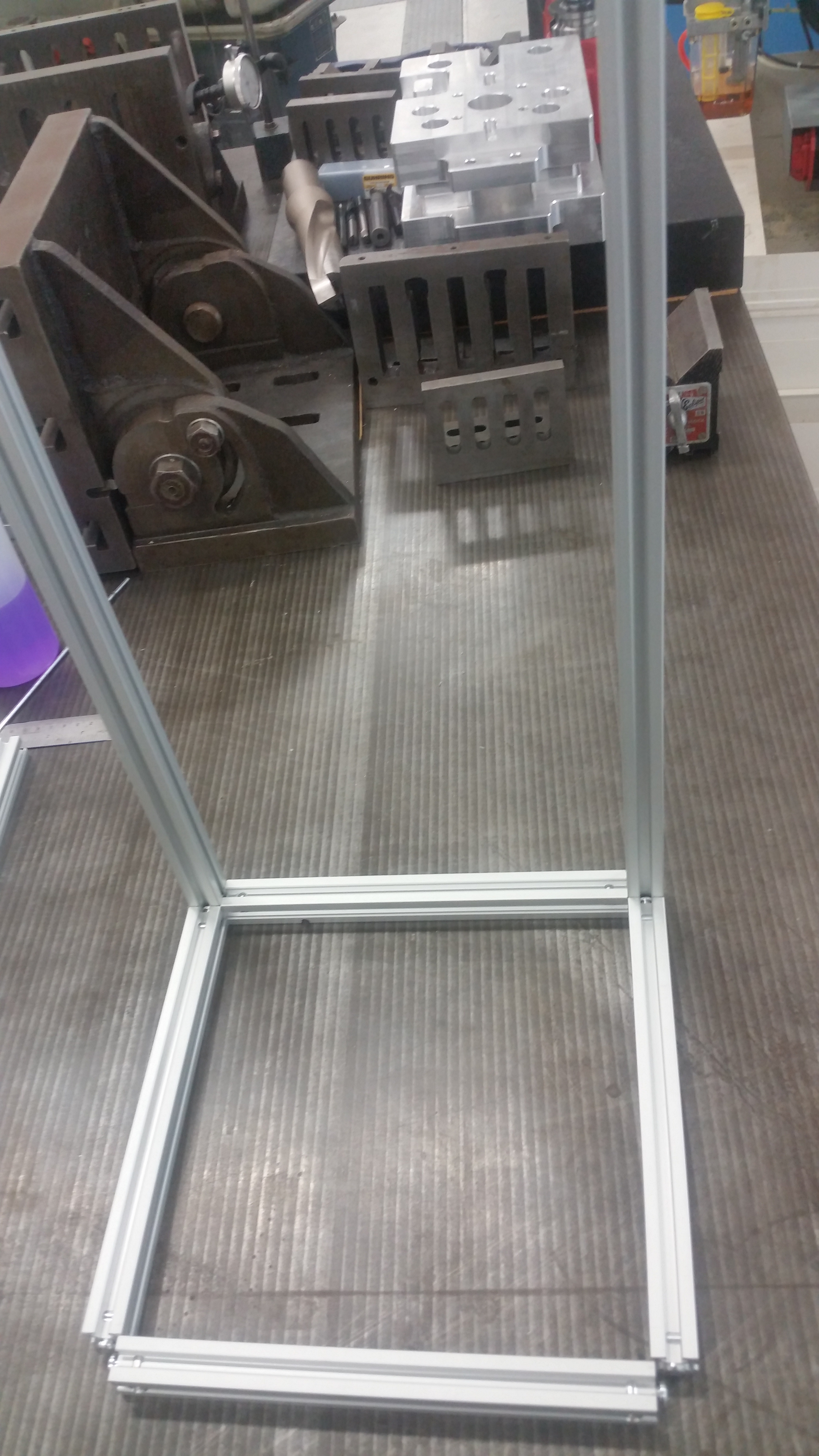

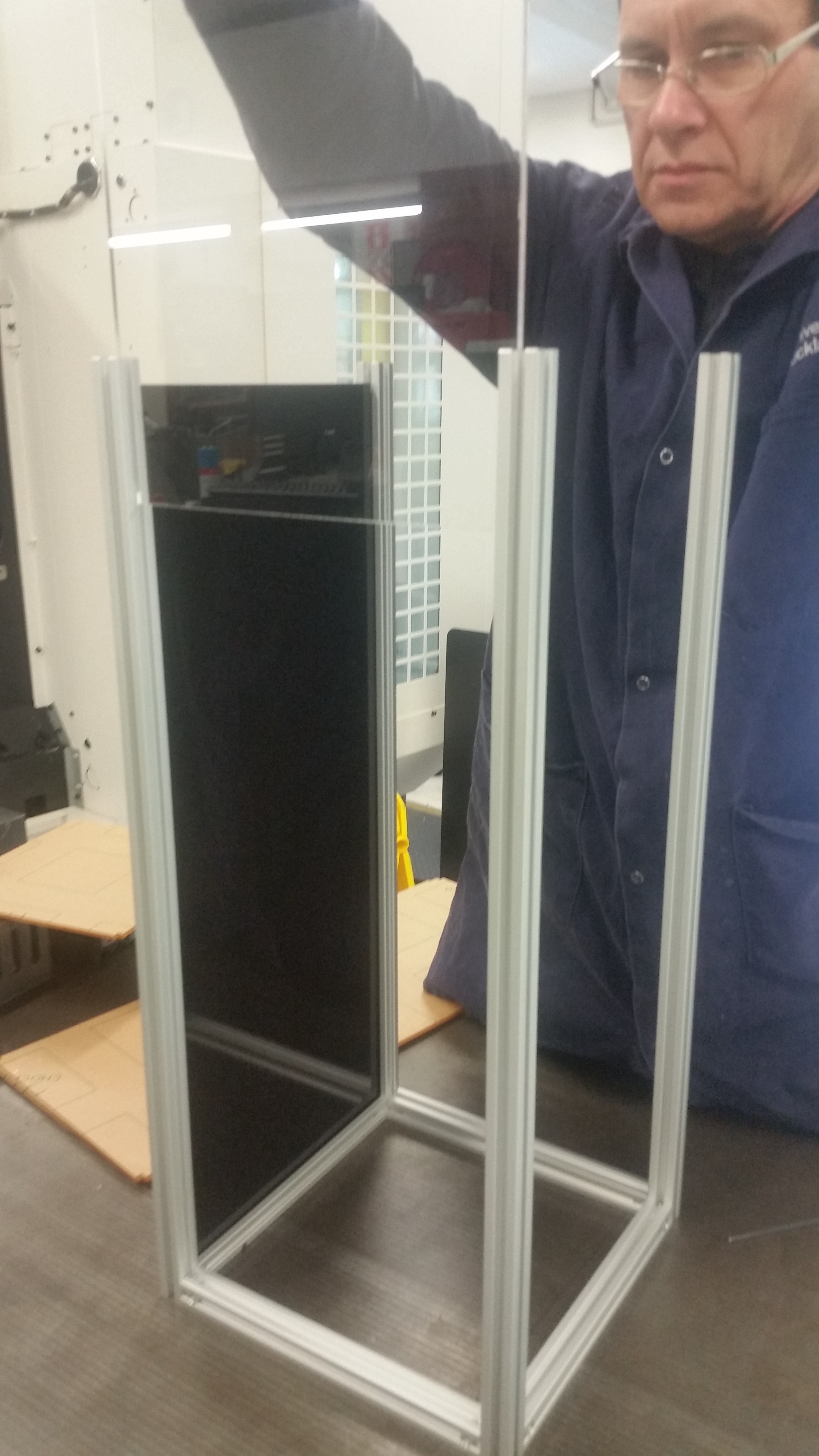


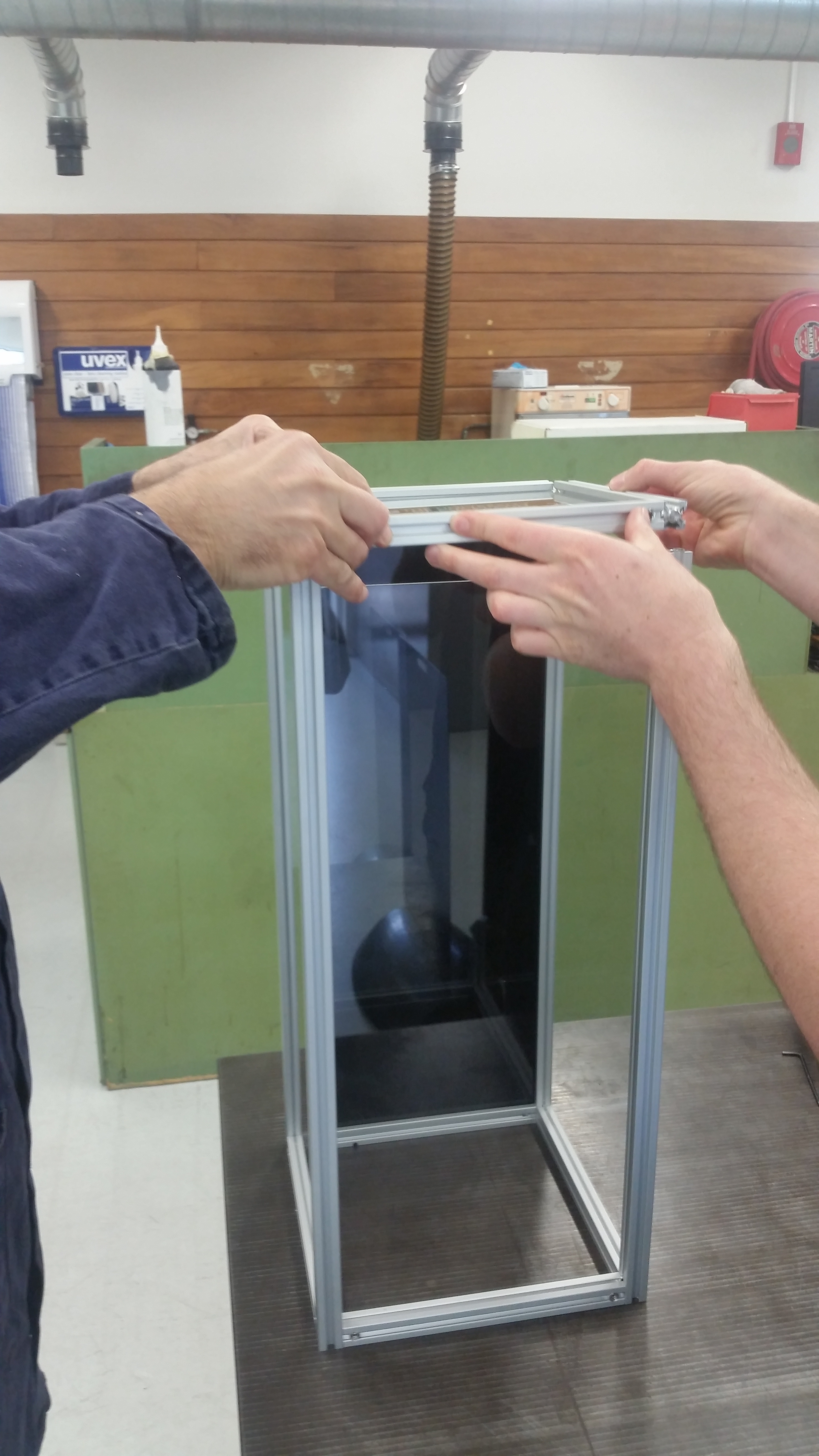
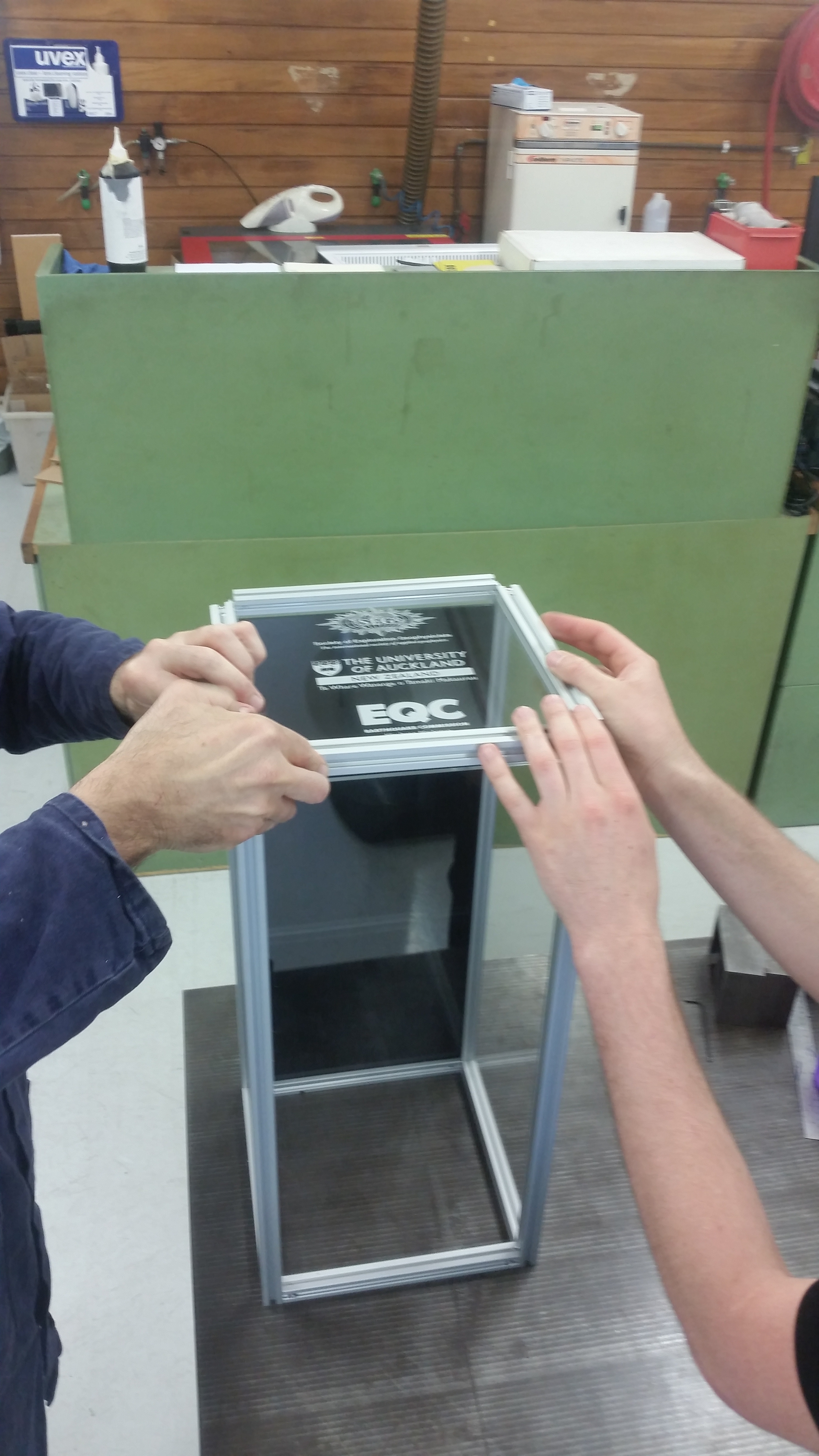

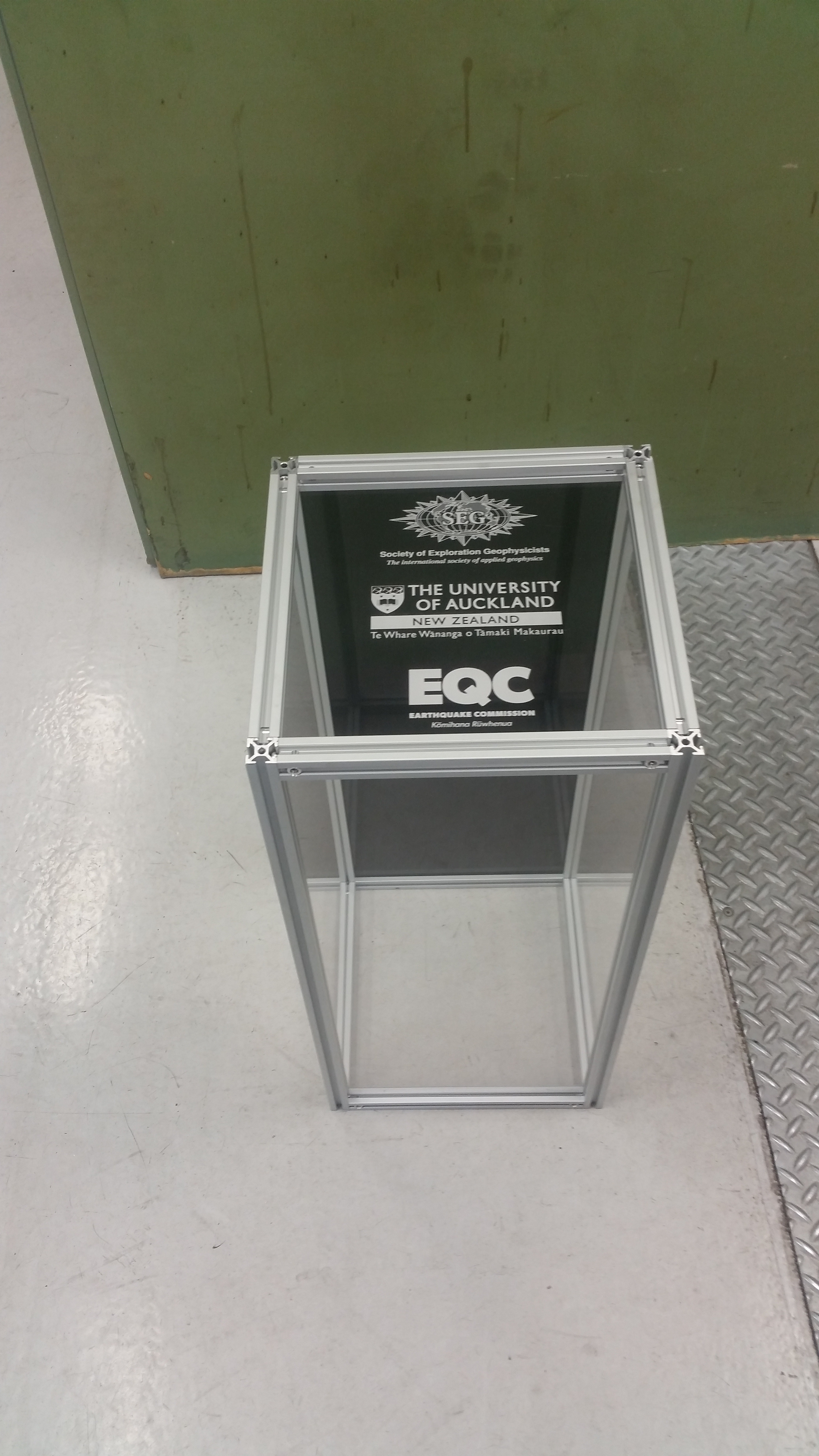
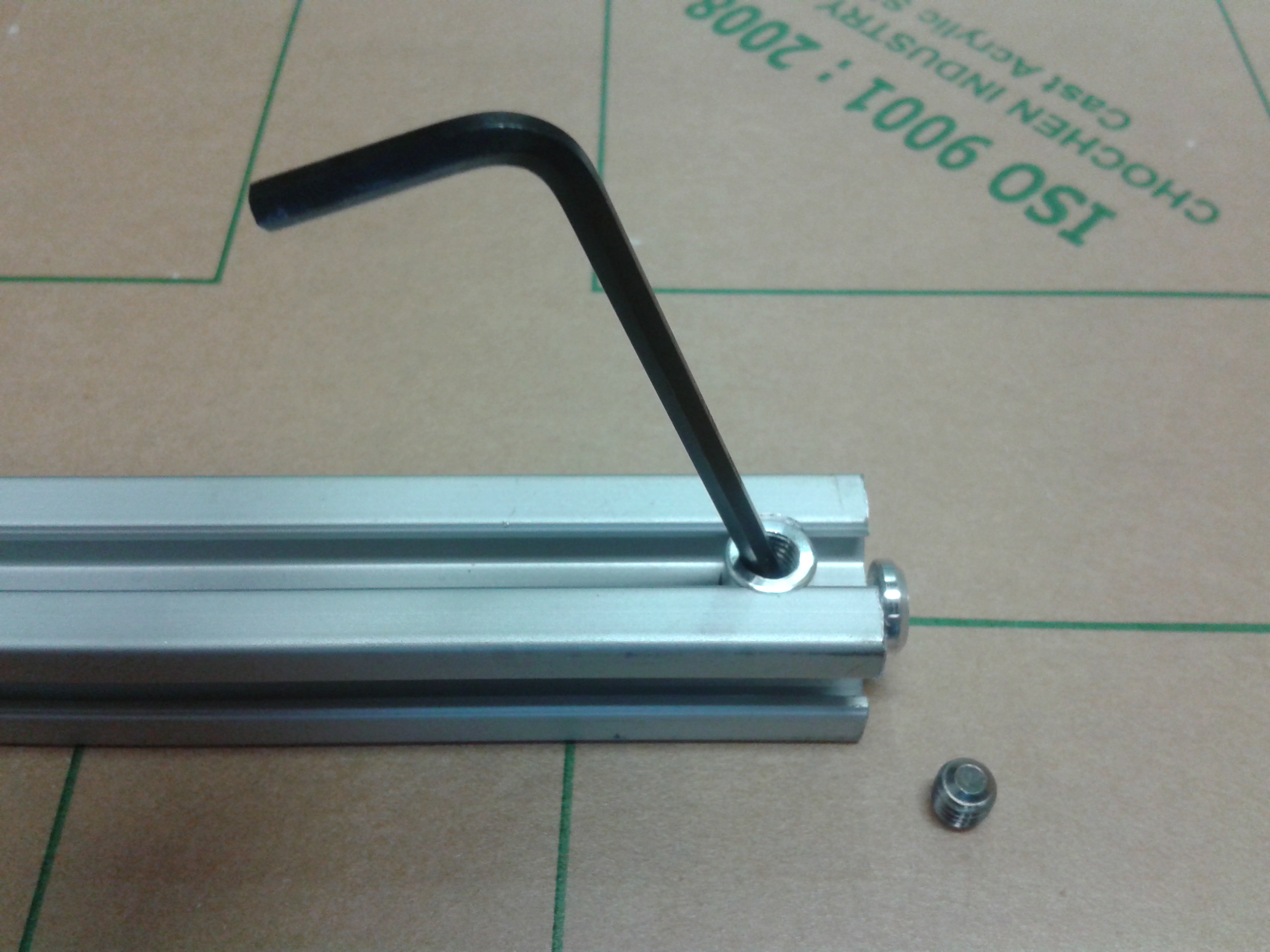
Click on the images for more detail and a short description.Once assembled, it is recommended to fasten the completed case to a wall.
Thank you Mark, Trevor, Steve and all others from the Science and Engineering Workshop!